How Learn Excel can Save You Time, Stress, and Money.

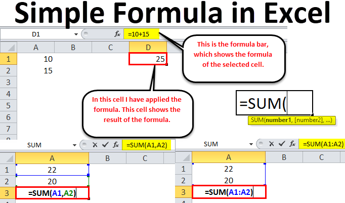
By pressing ctrl+change+center, this will certainly calculate and also return value from numerous arrays, as opposed to just individual cells included to or increased by each other. Determining the sum, item, or ratio of specific cells is very easy-- just utilize the =SUM formula as well as go into the cells, values, or variety of cells you intend to perform that math on.

If you're looking to discover overall sales revenue from a number of marketed units, for instance, the selection formula in Excel is best for you. Here's just how you 'd do it: To start utilizing the selection formula, kind "=SUM," as well as in parentheses, get in the very first of 2 (or three, or four) series of cells you would love to increase together.

This stands for multiplication. Following this asterisk, enter your 2nd series of cells. You'll be increasing this 2nd variety of cells by the first. Your progression in this formula should now resemble this: =AMOUNT(C 2: C 5 * D 2:D 5) Ready to press Enter? Not so quick ... Because this formula is so complicated, Excel gets a various key-board command for arrays.

This will certainly identify your formula as a variety, wrapping your formula in support personalities as well as effectively returning your item of both arrays integrated. In profits computations, this can reduce down on your effort and time dramatically. See the final formula in the screenshot over. The COUNT formula in Excel is denoted =MATTER(Begin Cell: End Cell).

For instance, if there are eight cells with entered values between A 1 and A 10, =COUNT(A 1: A 10) will return a value of 8. The COUNT formula in Excel is particularly useful for big spread sheets, in which you desire to see the amount of cells include real entrances. Don't be tricked: This formula won't do any type of mathematics on the values of the cells themselves.

A Biased View of Excel Jobs

Utilizing the formula in bold above, you can easily run a count of active cells in your spreadsheet. The result will certainly look a something similar to this: To perform the ordinary formula in Excel, enter the worths, cells, or range of cells of which you're calculating the average in the style, =STANDARD(number 1, number 2, and so on) or =AVERAGE(Start Value: End Value).

Discovering the standard of a series of cells in Excel keeps you from having to locate specific sums and after that performing a different division formula on your total. Utilizing =STANDARD as your preliminary message access, you can allow Excel do all the help you. For reference, the standard of a group of numbers is equal to the amount of those numbers, split by the variety of products in that team.

This will certainly return the sum of the values within a desired variety of cells that all satisfy one criterion. For instance, =SUMIF(C 3: C 12,"> 70,000") would return the amount of worths between cells C 3 as well as C 12 from only the cells that are greater than 70,000. Let's say you intend to establish the revenue you produced from a checklist of leads who are linked with particular area codes, or compute the amount of particular employees' salaries-- yet only if they fall above a particular quantity.

With the SUMIF function, it does not need to be-- you can quickly include up the amount of cells that fulfill certain criteria, like in the salary instance above. The formula: =SUMIF(array, criteria, [sum_range] Variety: The variety that is being evaluated utilizing your standards. Criteria: The criteria that identify which cells in Criteria_range 1 will certainly be added with each other [Sum_range]: An optional variety of cells you're mosting likely to build up along with the initial Array entered.

In the instance listed below, we wanted to calculate the sum of the wages that were more than $70,000. The SUMIF function included up the dollar amounts that surpassed that number in the cells C 3 via C 12, with the formula =SUMIF(C 3: C 12,"> 70,000"). The TRIM formula in Excel is represented =TRIM(message).

Some Known Questions About Learn Excel.

For instance, if A 2 consists of the name" Steve Peterson" with undesirable rooms prior to the given name, =TRIM(A 2) would certainly return "Steve Peterson" with no areas in a brand-new cell. Email and also submit sharing are fantastic tools in today's work environment. That is, till among your coworkers sends you a worksheet with some truly funky spacing.

As opposed to fastidiously removing as well as including spaces as required, you can tidy up any type of uneven spacing using the TRIM feature, which is used to eliminate additional areas from data (other than for single areas in between words). The formula: =TRIM(text). Text: The message or cell from which you intend to eliminate spaces.

To do so, we entered =TRIM("A 2") right into the Formula Bar, and also replicated this for each and every name listed below it in a brand-new column beside the column with unwanted areas. Below are a few other Excel formulas you could locate useful as your information management needs grow. Let's claim you have a line of text within a cell that you wish to damage down into a few different sectors.

Purpose: Used to extract the first X numbers or characters in a cell. The formula: =LEFT(message, number_of_characters) Text: The string that you wish to draw out from. Number_of_characters: The number of characters that you wish to extract starting from the left-most character. In the instance listed below, we entered =LEFT(A 2,4) into cell B 2, as well as replicated it right into B 3: B 6.

Objective: Utilized to draw out characters or numbers in the center based upon setting. The formula: =MID(message, start_position, number_of_characters) Text: The string that you wish to remove from. Start_position: The placement in the string that you want to start removing from. For example, the first placement in the string is 1.

Learn Excel for Dummies

In this example, we went into =MID(A 2,5,2) right into cell B 2, and duplicated it right into B 3: B 6. That allowed us to draw out both numbers beginning in the fifth position of the code. Function: Utilized to extract the last X numbers or characters in a cell. The formula: =RIGHT(text, number_of_characters) Text: The string that you wish to extract from.

excel formulas not showing result excel formulas won't update excel formulas not